Political information flow and management guidance

Political information flow and management guidance with Dane Christensen, Beverly Walther, and Laura Wellman.

Here’s the abstract:

We examine whether politically active firms play a role in disseminating political information via their management guidance. We use multiple proxies based on campaign financing activity or the presence of a government affairs office to capture whether a firm is politically active. We find that politically active firms are more likely to issue management guidance overall, and especially when the government is a key customer of the firm. Further, relative to politically inactive firms, the guidance released by politically active firms is more likely to discuss government policies. In addition to using numerous econometric techniques to address self-selection concerns, we examine the timing of when guidance is issued. We find that politically active firms are more likely to issue guidance prior to the public revelation of government policy decisions. Collectively, these findings suggest that the privileged information firms obtain through their political activities is shared with investors through voluntary disclosures.

The main results of this paper fit nicely into our field’s mental models of how evidence should be developed and presented.

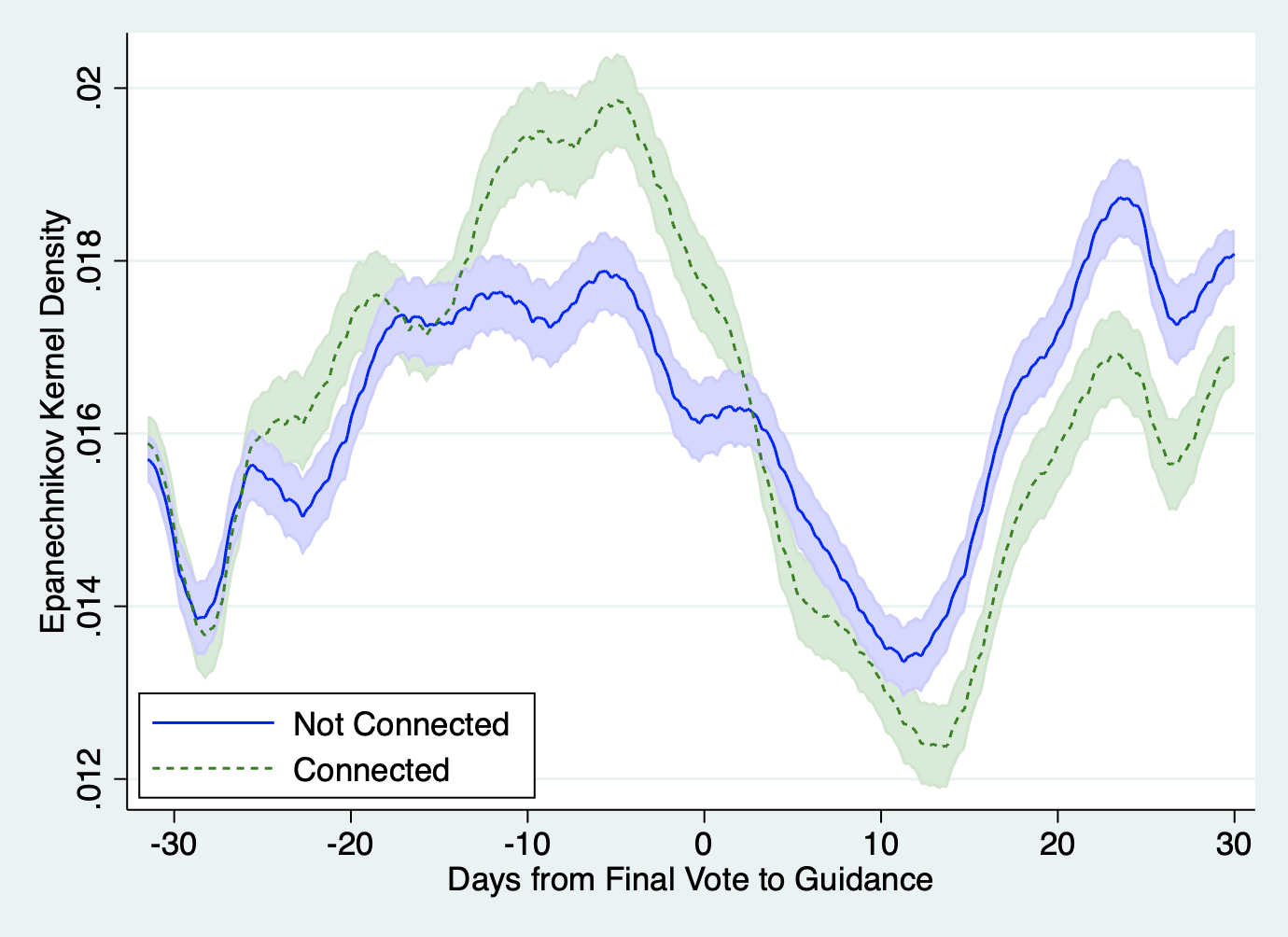
To make this graph we use kdens and twoway rarea in Stata. The steps for this weren’t obvious to me initially.

First load the data and label the variable of interest:

use "./timeToBillData.dta", clear
lab var timeToBill "Days from Final Vote to Guidance"

Second, estimate the density function for the non-connected group with a confidence interval

* not connected
kdens timeToBill if Connected == 0 & /// non-connected
		GUIDE == 1 & /// issue guidance
        !mi(lobbycount) & lobbycount>0 & /// peers lobby on this bill
		mi(timeToEA) & /// not bundled with an earnings announcement
        month < 1 & month > - 2 , /// limits to month -1 and 0
		ll(-31.5) ul(30) /// set the limits (+/- 30 days)
        /*kernel(epanechnikov)*/ /// epanechnikov kernel is the default
        reflection /// determines the shape at the bounds
        bw(n) /// bn(n) lets this data define the bins
		gen(d1 x1) /// saves the line
        ci(ci1_1 ci1_2) // saves the confidence interval

Third, estimate the density function for the connected group with a confidence interval

kdens timeToBill if Connected == 1 & /// non-connected
		GUIDE == 1 & /// issue guidance
        !mi(lobbycount) & lobbycount>0 & /// peers lobby on this bill
		mi(timeToEA) & /// not bundled with an earnings announcement
        month < 1 & month > - 2 , /// limits to month -1 and 0
		ll(-31.5) ul(30) /// set the limits (+/- 30 days)
        /*kernel(epanechnikov)*/ /// epanechnikov kernel is the default
        reflection bw(5.2560433) /// here we apply the bin from Connected=0 group
		gen(d0 x0) /// saves the line
        ci(ci0_1 ci0_2) // saves the confidence interval

Finally, plot the estimated density functions and their confidence intervals:

twoway rarea ci0_1 ci0_2 x0 , color(green*.2) || ///
	rarea ci1_1 ci1_2 x1 , color(blue*.2) || ///
	line d1 x1, lc(blue) || line d0 x0, lc(green) lp(shortdash) ///
	legend(order(3 "Not Connected" 4 "Connected") pos(7) ring(0) col(1)) ///
	xlabel(-30(10)30)  ytitle("Epanechnikov Kernel Density")

… and save the graph if you like:

graph export "./Tabs/F1_MAIN.png" , replace

Arthur Morris