Tax Shields and Net-of-tax returns on real and financial assets
Key concepts from last time
- Assets, investments, and projects all have different pre-tax returns ($r$).
- Tax rates ($t$) vary across individuals, jurisdictions, organizations, and assets.
Examples of 2.
- HK individual income tax ranges from 2% to 17%
- HK corporate tax is 16.5%
- US individual income tax ranges from 10% to 35%
- Mortgage interest is not taxed.
- US corporate tax rate was 35% until 2017, now 21%
- Investments (depreciation) are tax deductible
- Interest payments are tax deductible
- Note: non-Hong Kong tax laws are important for Hong Kong accountants, because these laws are often the reason why your clients/employers are doing business in Hong Kong.
Key concepts from last time
- Assets, investments, and projects all have different pre-tax returns ( $r$ ).
- Tax rates ( $t$ ) vary across individuals, jurisdictions, organizations, and assets.
- pre-tax returns of $r$ correspond to post-tax returns of $r(1-t)$
- for simple assets like savings accounts, money market funds and mutual funds.
Notice some thing similar for more complex assets
| Instrument | <div style="width:400px">Annualized Return</div> | |
|---|---|---|
| I. | Money Market Fund | $r(1-t)$ |
| II. | SPDA | $[(1+r)^{n}(1-t)+t]^{1/n} -1$ |
| III. | Mutual Fund | $r(1 - g)$ |
| IV. | Foreign Corporation | $[(1+r)^{n}(1-g)+g]^{1/n} -1$ |
| V. | Insurance Policy | $r$ |
| VI. | Pension | $r$ |
- Note: SPDAs and “Foreign” Corporations differ because taxes are paid on the income when you end the position.
- Note: That these are ‘annualized’ rates meaning the rate of return for each year.
- $r$ is the interest rate, $t$ is the income tax rate, and $g$ is the capital gains rate.
Key concepts from last time
- Assets, investments, and projects all have different pre-tax returns ($r$).
- Tax rates $t$ vary across individuals, jurisdictions, organizations, and assets.
- pre-tax returns $r$ correspond to post tax returns $r(1-t)$
- When preferential tax treatment increases demand for a tax favored asset it’s price increases. This price change is an implicit tax.
- When tax payers use organizational forms like pensions and insurance policies to avoid taxes it is called organizational form arbitrage.
- When high-tax tax payers issue taxable debt to finance the purchase of tax free debt (e.g. municipal bonds in the US) issued by low-tax tax payers (e.g. US non-profit universities) it is called clientele arbitrage.
Let’s look at the case (only 4:30 section)
- We are using an SPDA to illustrate a context in which a normal investor could implement a strategy like this.
- No need to memorize the SPDA formula.
- When comparing two options, always think about the revenue and costs that are unique to each scenario.
Now back to net-of-tax returns
Suppose there is a riskless financial asset that costs one dollar at the beginning of the period and pays $1 + r$ dollars at the end of every period. The difference, $r$, is taxed at rate $t$.
Thus, it is possible to borrow and lend at the after-tax rate of $r(1 - t)$ per period.
There is also a real asset costing $x > 0$. The asset produces a riskless pretax cash flow of $k$ in perpetuity at the end of each period.
Tax Treatment of Depreciation:
For tax purposes, the original cost of the asset may be depreciated straight line at rate $0 \leq d \leq 1$. Taxable income for any period is the pre-tax cash flow less the depreciation.
But wait!?!? Didn’t you just tell us not to consider depreciation?
- Why are we including depreciation?
- Notice where we include depreciation in the next equation!
Tax is paid at rate $t$, so that at the end of the first period, the net-of-tax cash flow is
\[k-t(k-dx)\]- $k$ is the return on the investment, $d$ is the depreciation rate, and $x$ is the investment.
Depreciation is impacting cash flow through it’s impact on the taxes you pay!
Tax Treatment of Depreciation:
We can rewrite the net-of-tax cash flow equation above as follows:
\[k(1-t) + dtx\]Now lets write down the cash flows from this project, and discount them.
What are the cash flows?
The cash outflow $x$ to acquire the asset is not tax deductible, so the first cash flow is just:
\[-x\]What are the cash flows?
- The second set of cash flows are the net-of-tax cash flows over the depreciable life of the asset discounted back to time zero at the after-tax rate of return
- $1/d$ is the number of periods you depreciate. e.g. if $d=.25$ then $1/d=4$ years
- the numerators are discounting cash flows relative with $r$ adjusted for $t$ you might recognize the formula from the previous lecture’s handout!
What are the cash flows?
The final set of cash flows we need to consider are then net-of-tax cash flows from the asset after the asset is fully depreciated.
\[\sum^{\infty}_{n=1+1/d}\frac{k(1-t)}{[1+r(1-t)]^{n}}\]- $1/d$ is the number of periods you depreciate. e.g. if $d=.25$ then $1/d=4$ years
- the numerators are discounting cash flows relative with $r$ adjusted for $t$ you might recognize the formula from the previous lecture’s handout!
So the total net-of-tax present value of these cash flows at the end of the first period is: \(-x + \sum^{1/d}_{n=1}\frac{k(1-t)+dtx}{[1+r(1-t)]^{n}}+\sum^{\infty}_{n=1+1/d}\frac{k(1-t)}{[1+r(1-t)]^{n}}\)
- $1/d$ is the number of periods you depreciate. e.g. if $d=.25$ then $1/d=4$ years
- the numerators are discounting cash flows relative with $r$ adjusted for $t$ you might recognize the formula from the previous lecture’s handout!
This quantity can be rewritten as follows:
\[-x+\frac{k}{r}+\frac{dtx}{r(1-t)}\Big(1-[1+r(1-t)]^{-1/d}\Big)\]This is using the annuity and perpetuity formulas.
Each of these terms has an important meaning:
\[-x+\frac{k}{r}+\frac{dtx}{r(1-t)}\Big(1-[1+r(1-t)]^{-1/d}\Big)\]The first term is the cost of the asset again.
Each of these terms has an important meaning:
\[-x+\frac{k}{r}+\frac{dtx}{r(1-t)}\Big(1-[1+r(1-t)]^{-1/d}\Big)\]The second term is the present value of the perpetual pre-tax cash flow from the asset, $k$, capitalized at the pre-tax rate, $r$. Note that this is the same as the after tax cash flow, $k(1-t)$, capitalized at the after tax discount rate, $r(1-t)$.
Each of these terms has an important meaning:
\[-x+\frac{k}{r}+\frac{dtx}{r(1-t)}\Big(1-[1+r(1-t)]^{-1/d}\Big)\]- The final term is the present value of the reduction in tax payments afforded by the depreciation deduction (often called the tax shield).
- Notice that this term has the same form as the present value of an annuity of $dtx$ for $1/d$ periods discounted at rate $r(1-t)$.
-
This is the only term where tax factors $d$ and $t$ play a role.
- If either the depreciation rate or the tax rate is zero, then the before tax and net-of-tax present values are the same.
-
If $d$ and $t$ are both positive then the value of the tax shield provided by depreciation is also positive. The value of the shield increases with both $d$ and $t$.
- If either the depreciation rate or the tax rate is zero, then the before tax and net-of-tax present values are the same.
- If $d$ and $t$ are both positive then the value of the tax shield provided by depreciation is also positive. The value of the shield increases with both $d$ and $t$.
- When tax depreciation is immediate, i.e., $d=1$, then the tax shield is
- This value can be substantial. Consider an investment that may be deducted fully from taxes in the year it is made, such as advertising. For $t=30\%$ and $r=10\%$, the tax shield is 28\% of the cost of the asset!
Let’s do some plotting to get a sense of this relationship
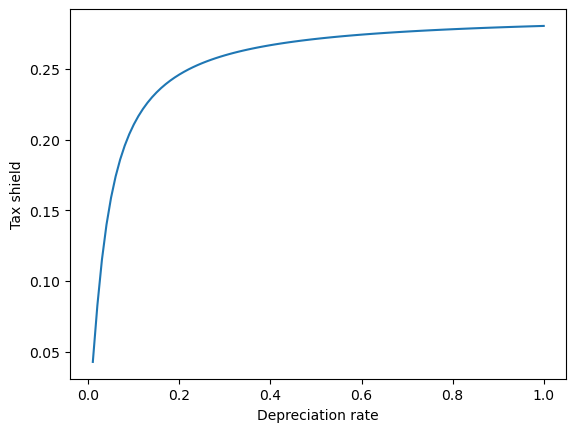
\[\frac{dtx}{r(1-t)}\Big(1-[1+r(1-t)]^{-1/d}\Big)=x\frac{t}{1+r(1-t)}\]First let’s plot the value of the tax shield as a function of the depreciation rate. Assume that $r=10\%$, and $t=30\%$
import matplotlib.pyplot as plt
import numpy as np

def tax_shield(d,t,r,x=1):
    first_term = (d*x*t)/(r*(1-t))
    second_term = 1-(1+r*(1-t))**(-1/d)
    return first_term*second_term
First let’s plot the value of the tax shield as a function of the depreciation rate. Assume that $r=10\%$, and $t=30\%$
D = np.linspace(0.01,1,100)
plt.plot(D,tax_shield(D,t=0.3,r=0.1))
plt.xlabel('Depreciation rate')
plt.ylabel('Tax shield')
plt.show()
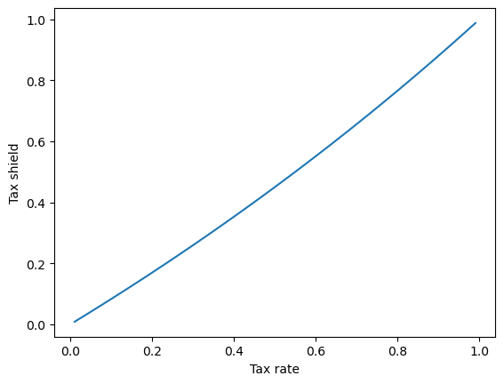
First let’s plot the value of the tax shield as a function of the depreciation rate. Now let’s plot the value of the tax shield as a function of the tax rate. Assume that $r=10\%$, and $d=30\%$
import warnings
warnings.filterwarnings('ignore')
T = np.linspace(0.01,1,100)
plt.plot(T,tax_shield(d=0.3,t=T,r=0.1))
plt.xlabel('Tax rate')
plt.ylabel('Tax shield')
plt.show()
One surprising conclusion that might be drawn from this analysis is that the net-of-tax present value of an investment is increasing in t.
That is, the higher the tax rate, the more attractive is the investment!
This might be the point!
- The depreciation tax shield makes investment more attractive.
- Investment encourages economic growth.
Questions:
- The statement above is a striking one. What must be held constant (and probably is not in real life) for it to be true?
- What condition defines equilibrium prices and returns on financial assets relative to real assets?
- What opportunities would you be able to exploit if you observed that prices and returns were not in equilibrium?
- What effect would your actions tend to have on prices and returns?
- Tricky question. What happens of the value of the depreciation tax shield as the tax rate, t approaches 100%? What is the intuition behind this result?
Questions:
- The statement above is a striking one. What must be held constant (and probably is not in real life) for it to be true?
- The demand for real assets! (implicit tax)
- Government spending may crowd out other types of investment.
- Also returns to scale.
- What condition defines equilibrium prices and returns on financial assets relative to real assets?
- No risk-free return from converting one to the other (no arbitrage)
- What opportunities would you be able to exploit if you observed that prices and returns were not in equilibrium?
- Arbitrage!
- What effect would your actions tend to have on prices and returns?
- Push them back to equilibrium.
Questions cont’d:
- Tricky question. What happens to the value of the value of the depreciation tax shield as the tax rate, t approaches 100%? What is the intuition behind this result?
- 100% of the value of the asset is as a tax shield.
tax_shield(d=0.3,t=.999999999,r=0.1)
1.0000001100223055
# TODO: add a slide for the value of a tax shield in hong kong