Step-down method: Does the order matter?
Does the order matter?
- The costs allocated to Cars and Trucks differ by only $27,000 depending on whether telecommunications or IT is chosen first.
- The difference of $27,000 is less than 1 percent of the total costs allocated.
Does the order matter?
- However, very different incentives result depending on which method is used.
- Allocated costs are taxes, and taxes effect behavior.
- And these can lead to the Death Spiral if the tax is too high!
Illustration
- To illustrate lets expand the telecommunications and IT example.
- Suppose the allocation base in telecommunications is the number of telephones in each department, and
- in IT the allocation base is the number of gigabytes of disk space used.
Illustration
- Transfer prices are to be established for telephones and gigabytes.
- Allocated costs will be used to compute the transfer prices.
The allocation bases
| |
Allocation base |
| Telecomm |
3,000 Telephones |
| IT |
12 million gigabytes |
Cost allocated per phone
Number of phones
| |
Direct |
Step, Telecomm first |
Step, IT first |
| Telecoms |
– |
– |
– |
| IT |
– |
20% $\times$ 3,000 = 600 |
– |
| Cars |
40% $\times$ 3,000 = 1,200 |
40% $\times$ 3,000 = 1,200 |
40% $\times$ 3,000 = 1,200 |
| Trucks |
30% $\times$ 3,000 = 900 |
30% $\times$ 3,000 = 900 |
30% $\times$ 3,000 = 900 |
| Phones |
2,100 |
2,700 |
2,100 |
- Note: that telecom is always ‘–’ here because we are considering how to allocate it’s costs. The in the ‘IT first’ column the telecom costs already include IT costs.
Cost allocated per phone
| |
Direct |
Step, Telecomm first |
Step, IT first |
| Cost per phone |
$2M/2,100 = |
$2M/2,700 = |
$3.765M/2,100 = |
| |
$ 952 |
$ 741 |
$1,793 |
| Number of phones: Cars |
1,200 |
1,200 |
1,200 |
| Telecoms charged to Cars |
$1.143 |
$0.889 |
$ 2.151 |
Does the order matter?
The order can lead to large changes in the ‘tax’ on the allocation base!
Cost allocated per Gigabyte of Storage
Number of Gigabytes of Storage
| |
Direct |
Step, Telecomm first |
Step, IT first |
| Telecoms |
– |
– |
25% $\times$ 12 = 3.0 |
| IT |
– |
– |
– |
| Cars |
35% $\times$ 12 = 4.2 |
35% $\times$ 12 = 4.2 |
35% $\times$ 12 = 4.2 |
| Trucks |
25% $\times$ 12 = 3.0 |
25% $\times$ 12 = 3.0 |
25% $\times$ 12 = 3.0 |
| Gigs |
7.2 |
7.2 |
10.2 |
- Note: that IT is always ‘–’ here because we are considering how to allocate it’s costs. The in the ‘Telecom first’ column the IT costs already include Telecom costs.
Cost allocated per Gigabyte of Storage
| |
Direct |
Step, Telecomm first |
Step, IT first |
| Cost per gig |
$6/7.2 = $0.833 |
$6.44/7.2 = $0.895 |
$6/10.2 = $0.588 |
| Number of gigs in Cars |
4.2 |
4.2 |
4.2 |
| IT charged to Cars |
$3.5 |
$3.759 |
$2.470 |
Cost allocated per Giga of storage (Millions except cost per Gb)
Consider the impact on behavior
- The sequence of service departments in the step-down method changes the costs of each service.
- Because the cost per phone (which represents the transfer price) varies depending whether or not it includes IT costs,
- the cost allocation scheme affects the decision of each department to add or drop phones.
- The same conclusions hold for the information technology department.
Does the order matter?
- Note the wide variation in cost per gigabyte.
- The cost varies from $0.588 per gigabyte under the step-down method with IT chosen first
- to $0.895 under the step-down method with telecommunications chosen first.
- The step-down method is an example of a sub-optimal status quo.
The central issues with the step-down method
- The sequence used is arbitrary and large differences can result in the cost per unit of service using different sequences.
- This creates an artificially low tax on the first department and an artificially high tax on the second department.
- Get this wrong and risk the death spiral.
- If you see the step-down method, find out why.
The reciprocal method
- Solves the problem by making the allocation simultaneously
Start by setting up the equations
Costs before allocation
| Consumer: |
Telecoms |
IT |
Cars |
Trucks |
Total |
| Provider: |
|
|
|
|
|
| Telecoms |
10% |
20% |
40% |
30% |
100% |
| IT |
25% |
15% |
35% |
25% |
100% |
| Cost incurred |
$2M |
$6M |
|
|
8M |
| Total to allocate: |
$T$ |
$I$ |
|
|
|
$I$ and $T$ are unknown because they include unallocated costs. We need to set up a system of equations and solve it to get these numbers.
Telecoms equation
- $T$ = Telecom Cost incurred, plus the portion of those costs that Telecom incurred, and the portion of IT that Telecom incurred.
- The equation is:
\[T = \$ 2M + 0.10 \times T + 0.25 \times I\]
- Notice that the $0.10 \times T$ term is decreasing the amount of $T$ to allocate, and $0.25 \times I$ is increasing it.
Now we algebra a little
- The equation simplifies to:
\(0.9\times T = \$ 2M + 0.25 \times I\)
\(T = \$ 2M/.9 + 0.25/.9 \times I\)
IT equation
- $I$ = IT cost incurred, plus the portion of those costs that IT itself incurred, and the portion of Telecom that IT incurred.
- The equation is:
\(I = \$6.0 + .20\times T + .15 \times I\)
\(.85I=\$6.0+.20\times T\)
- Notice that the $.15 \times I$ term is decreasing the amount of I to allocate.
Now algebra a little more
- Now we have two equations and two unknowns and we can solve by hand.
- As a proof of concept now we will use Google’s Colab platform to solve this
Pass the following to the colab notebook
# load symbolic python
import sympy as sp
# initialize I and T
I, T = sp.symbols('I, T')
Now define the equations
# - use the comma for '='
# - and simplify as little as you like
tel_eq = sp.Eq(
    2 + .25 * I , .9 * T
)
it_eq = sp.Eq(
    6 + .2 * T , .85 * I
)
Now ask for a solution
solution = sp.solve((tel_eq, it_eq),(I,T))
yields:
{I: 8.11188811188811, T: 4.47552447552448}
This approach is massively scalable
- This approach scales until google starts charging you! And after that until you run out of cash :)
- If we really wanted to have fun we could load weights and costs from a spreadsheet and do the calculation with matrix notation for hundreds of departments.
- Whatever the practice at a company, not knowing the reciprocal allocation is unwise.
add an equation to illustrate
I,T,J = sp.symbols('I,T,J')
tel_eq = sp.Eq(
    2 + .25 * I + .12 * J , .9 * T
)
it_eq = sp.Eq(
    6 + .2 * T + .38 * J , .85 * I
)
jt_eq = sp.Eq(
    .1 + .05 * I + .01 * T ,   J
)
solution = sp.solve((tel_eq, it_eq, jt_eq),(I,T,J))
numpy version that scales
for this we need a little more organization:
\(.25 \times I + .12 \times J - .9 \times T = -2\)
\(-.85 \times I + .38 \times J + .2 \times T = -6\)
\(.05 \times I - J + .01 \times T = -.1\)
then we can load this from a csv, or type the following
import numpy as np
lhs = np.array([
    [.25,.12,-.9],
    [-.85,.38,.2],
    [.05,-1,.01]
               ])
rhs = np.array(
    [-2,-6,-.1]
)
np.linalg.solve(lhs,rhs)
Service department cost allocation
| Consumer: |
Telecoms |
IT |
Cars |
Trucks |
Total |
| Provider: |
|
|
|
|
|
| Costs before allocation |
$2M |
$6M |
|
|
$8M |
Service department cost allocation
| Consumer: |
Telecoms |
IT |
Cars |
Trucks |
Total |
| Provider: |
|
|
|
|
|
| Costs before allocation |
$2M |
$6M |
|
|
$8M |
| Telecoms tot. to alloc. |
$(4.475) |
|
|
|
$(4.475) |
Service department cost allocation
| Consumer: |
Telecoms |
IT |
Cars |
Trucks |
Total |
| Provider: |
|
|
|
|
|
| Costs before allocation |
$2M |
$6M |
|
|
$8M |
| Telecoms tot. to alloc. |
$(4.475) |
|
|
|
$(4.475) |
| Amount allocated from Telecoms: |
$$4.475\times.10=$.448$ |
$$4.475\times.20=$.895$ |
$$4.475\times.40=$1.790$ |
$$4.475\times.30=$1.34.$ |
$4.475 |
| IT tot. to alloc |
|
$(8.112) |
|
|
$(8.112) |
| Amount allocated from IT: |
$$8.112\times.25=$2.028$ |
$$8.112\times.15=$1.217$ |
$$8.112\times.35=$2.839$ |
$$8.112\times.25=$2.028$ |
$8.112 |
| Total overhead allocated |
0.000 |
0.000 |
$4.629 |
$3.371 |
$8.000 |
Cost per phone
| |
Telecoms |
IT |
Cars |
Trucks |
Total |
| Allocated Telecoms costs (M) |
$ 0.448 |
$ 0.895 |
$1.790 |
$1.343 |
$ 4.475 |
| ÷ Number of phones |
300 |
600 |
1,200 |
900 |
3,000 |
| Cost per phone (M) |
$ 1,492 |
$ 1,492 |
$1,492 |
$1,492 |
$ 1,492 |
Cost per gig
| |
Telecoms |
IT |
Cars |
Trucks |
Total |
| Allocated IT costs |
$ 2.028 |
$ 1.217 |
$2.839 |
$2.028 |
$ 8.111 |
| ÷ Number of gigabytes (M) |
3.0 |
1.8 |
4.2 |
3.0 |
12.0 |
| Cost per gigabyte |
$ 0.676 |
$ 0.676 |
$0.676 |
$0.676 |
$ 0.676 |
Ask why
The fact that we observe infrequent use of the reciprocal method suggests
that accounting’s primary focus is not decision making, but rather some other
purpose such as financial reporting, or taxes.
Joint costs
Joint costs
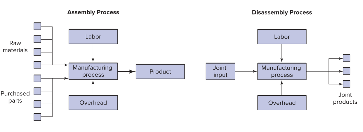
Joint costs and the death spiral
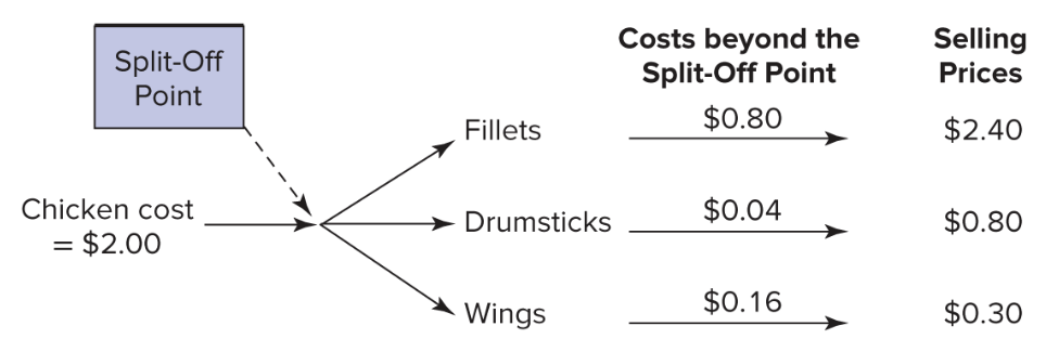
Chickens in the death spiral
- a chicken processor who buys live chickens and disassembles them into fillets, wings, and drumsticks.
- chickens cost $1.60 each.
- variable cost to process the chicken into parts is $0.40 per chicken.
- The joint cost per chicken is then $2.
Chickens in the death spiral
- separate processing is necessary to obtain marketable fillets, drumsticks, and wings.
- cost of $0.80 for fillets, $0.16 for wings, and $0.04 for drumsticks.
- the split-off point occurs where all joint costs have been incurred.
Chickens in the death spiral
| |
Total |
Fillets |
Drumsticks |
Wings |
| Cost alloc. on weight |
|
|
|
|
| Weight |
32 oz |
16 oz |
12 oz |
4 oz |
| % |
100% |
50% |
37.5% |
12.5% |
| Alloc’d cost |
$2.00 |
$1.00 |
$0.75 |
$ 0.25 |
| Profit |
|
|
|
|
| Sales |
$3.50 |
$2.40 |
$0.80 |
$ 0.30 |
| Costs beyond split-off point |
(1.00) |
(0.80) |
(0.04) |
(0.16) |
| Joint costs (from above) |
(2.00) |
(1.00) |
(0.75) |
(0.25) |
| Profit (loss) per chicken |
$0.50 |
$0.60 |
$0.01 |
$(0.11) |
Management decides to drop chicken wings.
Chickens in the death spiral
| |
Total |
Fillets |
Drumsticks |
| Cost alloc. on weight |
|
|
|
| Weight |
28 oz |
16 oz |
12 oz |
| % |
100% |
57.14% |
42.9% |
| Alloc’d cost |
$2.00 |
$1.14 |
$0.86 |
| Profit |
|
|
|
| Sales |
$3.20 |
$2.40 |
$0.80 |
| Costs beyond split-off point |
(0.84) |
(0.80) |
(0.04) |
| Joint costs (from above) |
(2.00) |
(1.14) |
(0.86) |
| Profit (loss) per chicken |
$0.36 |
$0.46 |
$(0.10) |
Management decides to drop chicken drumsticks.
Chickens in the death spiral
| |
Fillets |
| Weight |
16 oz |
| % |
100% |
| Alloc’d cost |
$2.00 |
| Profit |
|
| Sales |
$2.40 |
| Costs beyond split-off point |
(0.80) |
| Joint costs (from above) |
(2.00) |
| Profit (loss) per chicken |
$(0.40) |
Management decides that they were vegan all along and start selling cans of air from exotic locations.
So what’s wrong?
- the transfer of 25 cents to wings makes us think that we can avoid these costs if we stop making wings but we cannot
- the only costs and benefits considered in the decision to process further should be the actual costs and benefits that occur after we process further.
- consider the opportunity costs! What are the benefits foregone?
Net realizable value
- the benefit foregone if we do not process further
- this is the only metric we should use when considering elimination of joint products.
- other transfer prices may be used to align decisions with company goals.
Net realizable value
The NRV of chicken wings is $$0.30-$0.16=$0.14$