Standard Costs and Variances
Everything starts with a budget
- We can conduct variance analysis at any level of the organization.
- We can use decomposition of variances to isolate the causes.
- This tells us which parts of our forecasts were wrong.
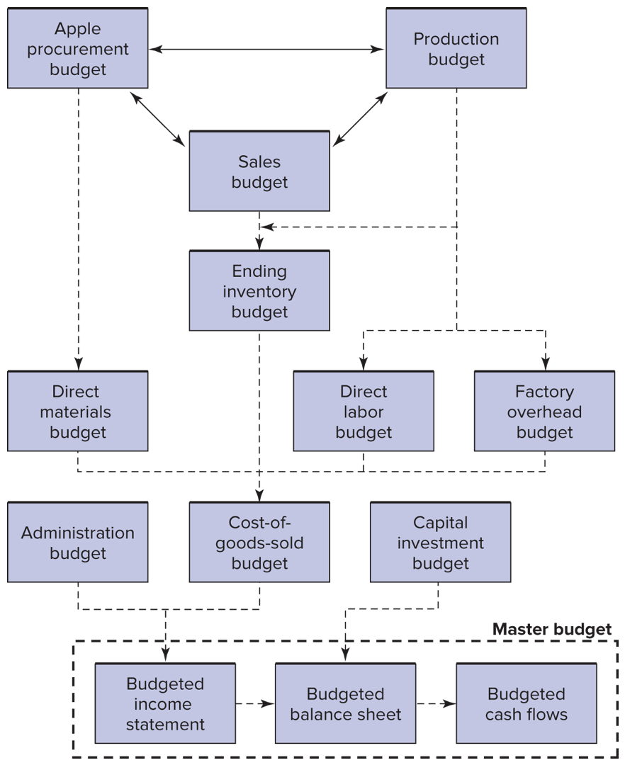
Logical flow
Example: Sandy Cove Bank
Sandy Cove Bank
- Sandy Cove is a new small commercial bank in Sandy Cove, Michigan.
- The bank limits interest rate risk by matching the maturity of its assets to the maturity of its liabilities.
- By maintaining a spread between interest rates charged and interest rates paid, the bank plans to earn a small income.
Sandy Cove Bank
- Management establishes a flexible budget based on interest rates for each department.
- The Boat and Car Loan Department offers five-year loans.
- It matches certificates of deposit (CDs) against car and boat loans.
Sandy Cove Bank
- Given all the uncertainty about interest rates, management believes that five-year savings interest rates could vary between 2 percent and 16 percent for the coming year. (Note: ‘Given’ in this sentence embeds a critical management accounting activity: forecasting.)
- The savings rate is the rate paid on CD savings accounts.
- The loan rate is the rate charged on auto and boat loans.
Sandy Cove Bank
- Expected new demand for fixed-rate, five-vear loans and the new supply of fixed-rate, five-year savings accounts at various interest rates.
| Loan Rate | Loan Demand | Savings Rate | Savings Supply |
|---|---|---|---|
| 6% | $12,100,000 | 2 | $ 4,700,000% |
| 7% | 10,000,000 | 3 | 5,420,000 |
| 8% | 8,070,000 | 4 | 8,630,000 |
| 9% | 6,030,000 | 5 | 9,830,000 |
| 10% | 4,420,000 | 6 | 11,800,000 |
- There are no loans from previous years. Note that the department maintains a 4 percent spread between loan and savings rates to cover processing, loan default, and overhead.
Sandy Cove Bank
- The amount of new loans granted is always the lesser of the loan demand and loan supply.
- For simplicity, this bank may lend 100 percent of deposits.
- In practice, this rate is set by policy makers and regulators not the bank itself.
Sandy Cove Bank
- Although rates are set nationally, the bank may pay or charge slightly different rates to limit demand or boost supply as needed in its local market.
- The Boat and Car Loan Department incurs processing, loan default, and overhead expenses related to these accounts.
Sandy Cove Bank
- The first two expenses vary, depending on the dollar amount of the accounts.
- The annual processing expense is budgeted to be 1.5 percent of the loan accounts.
- Default expense is budgeted at 1 percent of the amount loaned per year.
Sandy Cove Bank
- Again, loans and savings would ideally be the same.
- Overhead expenses are estimated to be $30,000 for the year, regardless of the amount loaned.
SCB Question 1
- Calculate the processing, loan default, and overhead expenses for each possible interest rate.
| Loan Rate | Loan Demand | Savings Rate | Savings Supply | New Loans |
|---|---|---|---|---|
| 6% | $12.1 M | 2% | $ 4.7 M | $ 4.7 M |
| 7% | 10 | 3% | 5.42 | 5.42 |
| 8% | 8.07 | 4% | 8.63 | 8.07 |
| 9% | 6.03 | 5% | 9.83 | 6.03 |
| 10% | 4.42 | 6% | 11.8 | 4.42 |
SCB Solution 1
| Loan Rate | Loan Demand | Savings Rate | Savings Supply | New Loans | Processing Expenses |
|---|---|---|---|---|---|
| 6% | $12.1 M | 2% | $ 4.7 M | $ 4.7 M | $70,500 |
| 7% | 10 | 3% | 5.42 | 5.42 | 81,300 |
| 8% | 8.07 | 4% | 8.63 | 8.07 | 121,050 |
| 9% | 6.03 | 5% | 9.83 | 6.03 | 90,450 |
| 10% | 4.42 | 6% | 11.8 | 4.42 | 66,300 |
- Processing is 1.5% of loan accounts
SCB Solution 1
| Loan Rate | Loan Demand | Savings Rate | Savings Supply | New Loans | Processing Expenses | Default Exp |
|---|---|---|---|---|---|---|
| 6% | $12.1 M | 2% | $ 4.7 M | $ 4.7 M | $70,500 | $47,000 |
| 7% | 10 | 3% | 5.42 | 5.42 | 81,300 | 54,200 |
| 8% | 8.07 | 4% | 8.63 | 8.07 | 121,050 | 80,700 |
| 9% | 6.03 | 5% | 9.83 | 6.03 | 90,450 | 60,300 |
| 10% | 4.42 | 6% | 11.8 | 4.42 | 66,300 | 44,200 |
- Default expense is budgeted at 1 percent of the amount loaned per year.
SCB Solution 1
| Loan Rate | Loan Demand | Savings Rate | Savings Supply | New Loans | Processing Expenses | Default Exp | Overhead Expenses |
|---|---|---|---|---|---|---|---|
| 6% | $12.1 M | 2% | $ 4.7 M | $ 4.7 M | $70,500 | $47,000 | $30,000 |
| 7% | 10 | 3% | 5.42 | 5.42 | 81,300 | 54,200 | 30,000 |
| 8% | 8.07 | 4% | 8.63 | 8.07 | 121,050 | 80,700 | 30,000 |
| 9% | 6.03 | 5% | 9.83 | 6.03 | 90,450 | 60,300 | 30,000 |
| 10% | 4.42 | 6% | 11.8 | 4.42 | 66,300 | 44,200 | 30,000 |
- These are the budgeted expenses, this is the foundation of financing plans to make sure that these resources are in place when they are needed.
- In this case it is the deposits that need to be in place for the lending to happen.
SCB Question 2
- Create an annual budgeted income statement for five-year loans and deposits for the Boat and Car Loan Department given a savings interest rate of 4 percent. Remember to match supply and demand.
| Interest income | $8,070,000 × 8%= | $645,600 |
| Interest expense | $8,070,000 × 4%= | 322,800 |
| Net interest income | $322,800 | |
| Fixed overhead | 30,000 | |
| Processing expense | 121,050 | |
| Default expense | 80,700 | |
| Net income | $ 91,050 |
SCB Question 3
- Table 2 shows the actual income statement for the Boat and Car Loan Department. Included are the actual loans and savings for the same period. Calculate the variances and provide a possible explanation.
| Budget | Actual | |
|---|---|---|
| Interest income | $645,600 | $ 645,766 |
| Interest expense | 322,800 | 314,360 |
| Net interest income | $322,800 | $ 331,406 |
| Fixed overhead | 30,000 | 30,200 |
| Processing expense | 121,050 | 130,522 |
| Default expense | 80,700 | 77,800 |
| Net income | $ 91,050 | $ 92,884 |
| Loans | 8,070,000 | $8,062,000 |
| Deposits | 8,070,000 | $8,123,000 |
SCB Solution 3
| Budget | Actual | Fav. (Unfav.) Variance | |
|---|---|---|---|
| Interest income | $645,600 | $ 645,766 | $ 166 |
| Interest expense | 322,800 | 314,360 | 8,440 |
| Net interest income | $322,800 | $ 331,406 | $ 8,606 |
| Fixed overhead | 30,000 | 30,200 | (200) |
| Processing expense | 121,050 | 130,522 | (9,472) |
| Default expense | 80,700 | 77,800 | 2,900 |
| Net income | $ 91,050 | $ 92,884 | 1,834 |
| Loans | 8,070,000 | $8,062,000 | $ (8,000) |
| Deposits | 8,070,000 | $8,123,000 | $(53,000) |
SCB Solution 3
- Even though loans were lower and deposits were higher than expected, interest income was higher and interest expense was lower than expected.
- The answer can be obtained by calculating the average interest rates earned and paid.
SCB Solution 3
- On $8,062,000 worth of loans, Sandy Cove earned $645,766 interest, or 8.01 percent (0.01 percent more than expected).
- Similarly, it paid only 3.87 percent (0.13 percent less) on deposits.
SCB Solution 3
- Therefore, the net interest income variance of $8,606 is a combination of two effects: the variance in the actual loans and deposits (quantity) and the variance in the interest rates (price).
- The combined effects are a favorable interest income variance, a favorable interest expense variance, and an overall favorable net interest income variance.
SCB Solution 3
- At a savings interest rate of 4 percent, there is an excess supply of deposits over demand for loans.
- The Boat and Car Loan Department lowered the interest rate on deposits to stem additional deposits.
SCB Solution 3
- The increase in the interest rate on loans can be attributed only to an increase in the demand for loans, which resulted in the department charging a slightly higher average interest rate.
- The higher processing expense could be related to the higher number of accounts processed and improvements in the default rate.
- That is, the favorable default expense could be attributed to an improved screening process-related to spending more on processing.
Terminology
Before we dig into understanding variances, we need to define a couple of terms.
Standards vs. Budgets
- Budgeted costs and standard costs are the same thing.
- You can think of a ‘budget’ as the entire financial and operational plan.
- You can think of the ‘standards’ as all of the individual forecasts that go into the budget.
- Though the words are used interchangeably.
Standards vs. Actuals
- Standards are our predictions (generated from our model of costs)
- Actuals are what we observe (generated by reality)
Note that this definition is related to the data selection issue on the mid-term.
Variance:
Total Variance = Actual Cost - Standard Cost
Decomposing Variances
Total Var. into Price & Quantity Vars
- Start with this:
Total variance is equal to actual cost minus standard cost.
Total Var. into Price & Quantity Vars
- Define a few variables:
| Symbol | Subscript | ||
|---|---|---|---|
| Total Variance | TV | Actual | a |
| Quantity | Q | Standard | s |
| Price | P |
- This is all we need to decompose any variance into it’s price and volume components.
Total Var. into Price & Quantity Vars
- Now we can rewrite this:
- Total Variance = Actual Cost - Standard Cost
- In terms of prices and quantities as this:
- TV = (Qa×Pa) − (Qs×Ps)
- and do a little bit of algebra to do the decomposition.
Note: I’ll give you the relationship above, and you can either memorize or derive the other forms.
Decomposition:
The algebra:
- Goal: Write the rhs. so that one term includes the change error in
P and the other includes the
error in Q.
- TV = (Qa×Pa) − (Qs×Ps)
- Start by adding and subtracting (Ps×Qa)
- TV = (Qa×Pa) + [(Ps×Qa)−(Ps×Qa)] + (Qs×Ps)
Does (Ps×Qa) have real world meaning?
- Ps is the standard or budgeted price.
- Qa is the actual quantity.
- So Ps × Qa
is a flexible budget!
- (Or at least it’s one line from a flexible budget.)
The algebra:
- TV = [(Qa×Pa)−(Ps×Qa)] + [(Ps×Qa) − (Qs×Ps)
- TV = [Qa(Pa−Ps)] + [Ps(Qa−Qs)]
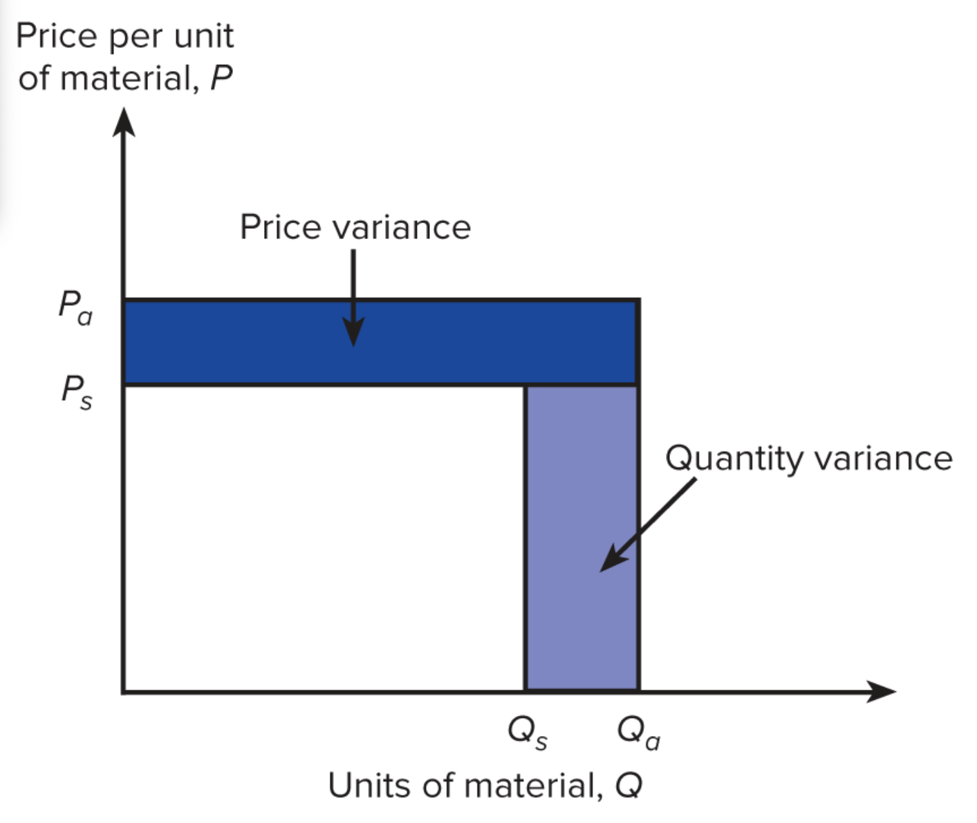
The Price and Quantity Variances
The Price and Quantity Variances
TV = [Qa(Pa−Ps)] + [Ps(Qa−Qs)]
- Now we have TV as a function of the error in P (Pa−Ps) and the error in Q (Qa−Qs).
- Multiplying the error in P by the actual quantity gives us the portion of TV that is due to the error in P.
The Price and Quantity Variances
- Multiplying the error in Q by the forecasted (budgeted, or standard) quantity gives us the portion of TV that is due to the error in Q.
The intuition behind this decomposition is critical.
The Price and Quantity Variances
TV = Qa(Pa−Ps) + Ps(Qa−Qs)
| Total Variance | Price Variance | Volume Variance |
|---|---|---|
| TV | [Qa(Pa−Ps)] | [Ps(Qa−Qs)] |
Three variance decompositions
This is the general form: TV = [Qa(Pa−Ps)] + [Ps(Qa−Qs)] now we’ll consider specific versions.
Direct Labor Variance
| Actual DL Cost | Flexible Budget | Standard DL Cost | |
|---|---|---|---|
| General Form | Pa × Qa | Ps × Qa | Ps × Qs |
We have other terms for the price and quantity of labor!:
- Price ($P) → Wage (W)
- Quantity → Hours
Direct Labor Variance
| Total Variance | Actual DL Cost | Flexible Budget | Standard DL Cost |
|---|---|---|---|
| (Ha×Wa) − (Ws×Hs) | Wa × Ha | Ws × Ha | Ws × Hs |
Direct Labor Variance
| Total Variance | Wage Variance | Efficiency Variance |
|---|---|---|
| (Ha×Wa) − (Ws×Hs) | Wa × Ha − Ws × Ha | Ws × Ha − Ws × Hs |
| [Ha(Wa−Ws)] + [Ws(Ha−Hs)] | Ha(Wa−Ws) | Ws(Ha−Hs) |
Why is the “Volume Variance” called the “Efficiency Variance” when we are talking about labor?
What might DLVs mean?
Large variances in either direction indicate performance is not as planned, due to either poor planning, poor management, or random fluctuation.
What might DLVs mean?
- Unfavorable wage variance
- Workers were not available at lower rates
- Unfavorable wage variance with favorable efficiency variance
- Higher-paid workers performed work more efficiently
- Favorable wage variance with unfavorable efficiency variance
- Lower-paid workers performed work less efficiently
Direct Materials Variance
| Actual DM Cost | Flexible Budget | Standard DM Cost | |
|---|---|---|---|
| General Form | Pa × Qa | Ps × Qa | Ps × Qs |
For materials we stick with the term “Price” and “Quantity”
Direct Materials Variance
| Total Variance | Actual DM Cost | Flexible Budget | Standard DM Cost |
|---|---|---|---|
| (Qa×Pa) − (Ps×Qs) | Pa × Qa | Ps × Qa | Ps × Qs |
| Total Variance | Price Variance | Quantity Variance |
|---|---|---|
| (Qa×Pa) − (Ps×Qs) | Pa × Qa − Ps × Qa | Ps × Qa − Ps × Qs |
| [Qa(Pa−Ps)] + [Ps(Qa−Qs)] | Qa(Pa−Ps) | Ps(Qa−Qs) |
Incentive Effects of Variances:
- Rewarding purchasing managers for favorable direct materials price variances creates an incentive for them to buy large quantities when price discounts are offered for high-volume purchases.
- Penalizing production managers for unfavorable labor efficiency variances encourages keeping labor busy producing more.
Incentive Effects of Variances:
- Mitigation of inventory building incentive
- Charge purchasing department for cost of holding inventory.
- Just-in-time (JIT) purchasing and production policies
A note on JIT:
- Mangerial accountants and consultants love JIT
- Toyota (and the whole Japanese Auto industry) is an often cited example.
- The 2011 Tohoku and Miyagi Earthquakes disrupted supply chains which lead to careful restructuring, and decreased reliance on pure just-in-time production.
A note on JIT:
- Nonetheless, JIT was still widely used and COVID 2019 disrupted these supply chains.
- The Invasion of Ukraine by the Russian military also disrupted supply chains.
- In all of these cases excess inventory proved immensely valuable.
Overhead Variance
Overhead Variance: Terms
- Overhead variances are slightly more complex, because in addition to predicting price and quantity we also have to predict overhead consumption (the overhead rate).
- This is a ‘meta’ prediction in the sense that it depends on several
other predictions:
- Consumption of the overhead
- Use of the underlying driver
- So when we observe an overhead variance, there are more things to explore.
Overhead Variance: Volume
- BV: Budgeted volume
- (also known as denominator volume)
- Estimated at the beginning of the year and used for calculating the overhead rate
- SV: Standard volume
- (also known as earned or allowed volume)
- (Output units completed) × (Standard input hours per output unit)
- Volume used to apply overhead to work-in-process inventory
- AV: Actual volume
- Actual hours or other input resource used during period
Overhead Variance: Volume Estimates
- Estimated budget volume influences overhead rate.
- Increasing budgeted volume (denominator) while holding total budgeted dollars constant (numerator) decreases the overhead rate.
- Expected volume to set budget
- Adjust expectation based on number of units forecast for next year.
- Rises and falls with business cycle
- Normal volume to set budget
- Forecast of long-run average annual production
- Does not change over business cycle
Flexible and Static Overhead Budgets:
For the sake of a simple example assume that the Toronto Engine Plant exists and has the following attributes:
| Forecast | |
|---|---|
| Fixed Overhead (FOH) | $1,350,000 |
| Variable Overhead (VOH) | $14 |
| Budgeted Volume (BV) | |
| (the driver is DLH) | 67,500 hours |
Remember that this “budgeted volume” is different than the “standard volume” though this distinction isn’t particularly clear given the way that we named things in the direct variances.
Flexible Overhead Budget (BOHFlex)
- Flexible overhead budget is the formula for budget forecast.
- BOHFlex = FOH + (VOH×BV)
- BOHFlex = $1, 350, 000 + ($14×BV)
Remember that Flexible Budgets are always formulas.
(Static) Overhead Budget
- Estimate budgeted overhead (BOH) dollars using a specific forecasted volume number (BV) and the flexible overhead budget formula.
- BOH = FOH + (VOH×BV)
- BOH = $1, 350, 000 + ($14×67,500hours)
- BOH = $2, 295, 000
Overhead Rate:
- This is the same sort of overhead rate that we’ve been thinking about with all of our allocations.
- Overhead rate is the total budgeted overhead dollars for the year divided by the budgeted volume for the year.
OHR = (BOH/BV) = (FOH/BV) + VOH OHR = ($2,295,000/67,000hours) = $1, 350, 000/67, 000hours + $14OHR = 34$$
The Overhead Rate Consists of Estimated:
- Fixed overhead $ per input hour (FOH / BV), and
- Variable overhead $ per input hour (VOH)
We need volume information!
Budgeted Volume
Budgeted Volume (Using Expected Volume)-Toronto Engine Plant’s Cylinder Boring Department
| Product | Expected Production | Standard Hours per Block | Budgeted Volume |
|---|---|---|---|
| 4-cylinder blocks | 25,000 blocks | 0.50 | 12,500 |
| 6-cylinder blocks | 40,000 blocks | 0.70 | 28,000 |
| 8-cylinder blocks | 30,000 blocks | 0.90 | 27,000 |
| Total | 95,000 blocks | ||
| Budgeted volume | 67,500 |
Actual and standard volumes:
| Product | Actual Production | Standard Hours per Block | Standard Volume | Actual Volume |
|---|---|---|---|---|
| 4-cylinder blocks | 27,000 blocks | 0.50 | 13,500 | 14,200 |
| 6-cylinder blocks | 41,000 blocks | 0.70 | 28,700 | 29,000 |
| 8-cylinder blocks | 28,000 blocks | 0.90 | 25,200 | 25,000 |
| Total | 96,000 blocks | |||
| Standard volume (SV) | 67,400 | |||
| Actual volume (AV) | 68,200 |
Volumes:
| Budgeted | Standard | Actual |
|---|---|---|
| 67,500 | 67,400 | 68,200 |
Overhead Allocated or Absorbed
- To allocate overhead we use the overhead rate and the standard volume.
- Standard Volume = Units of output ×
Standard input per output
- SV = 67,400 machine hours for 96,000 blocks
- Overhead absorbed = Overhead rate ×
Standard volume = OHR × SV
- Overhead absorbed = $34 × 67,400 machine hours = $2,291,600
Actual Overhead Cost:
$2,300,000
Total Overhead Variance
- Overhead variances occur when the actual overhead incurred does not equal the overhead absorbed or allocated.
Total Overhead Variance
Total Overhead Variance = Actual Overhead Costs - Overhead Absorbed AOH − (OHR×SV) = AOH − (OHR×SV)$2,300,000 - $2,291,600 = $8,400
Interpretation: - Overhead is ‘Underabsorbed’, if actual > absorbed - Overhead is ‘Overabsorbed’, if actual < absorbed
Decompose Overhead Variance
Decompose Overhead Variance
Total Overhead Variance = Actual Overhead - Overhead Absorbed
- Overhead spending variance = Actual overhead - Flexible budget at actual volume
- OSV = AOH - FB@AV
- Overhead efficiency variance = Flexible budget at actual volume - Flexible budget at standard volume
- OEV = FB@AV - FB@SV
- Overhead volume variance = Flexible budget at standard volume - Overhead Absorbed
- OVV = FB@SV - OA
Decompose Overhead Variance
| TOV | = | AOH | - | OA | ||||
|---|---|---|---|---|---|---|---|---|
| OSV | = | AOH | - | FB@AV | ||||
| OEV | = | FB@AV | - | FB@SV | ||||
| OVV | = | FB@SV | - | OA |
More detailed definitions:
| TOV | = | AOH | - | OHR × SV | ||||
|---|---|---|---|---|---|---|---|---|
| OSV | = | AOH | - | FOH+(VOH×AV) | ||||
| OEV | = | FOH+(VOH×AV) | - | FOH+(VOH×SV) | ||||
| OVV | = | FOH+(VOH×SV) | - | OHR × SV |